Some elements of Excel

To know the elements excel 2007 screen

• Office button: When clicked, this button opens the Office menu, from Which You Can open, save, print, and exit as well as the Excel Options button Enables you to change That Excel's default settings.
• Quick Access Toolbar: A small toolbar button next to the Office contains shortcuts for Some of the Most Common commands Such as Save, Undo, Redo and buttons. Also You Can Customize Quick Access Toolbar .
• Ribbon: A combination of old versions menu bar and toolbar, arranged a series of tabs Into ranging from Home-through View. Each tab contains buttons, lists, and commands.
• Name box: Displays the address of the current active cell in the WHERE you work worksheet.
• Formula Bar: Displays the address of the active cell on the left edge, and it shows you the current Also cell's contents.
• Worksheet area: This area contains all the cells of the current worksheet by column headings Identified, using letters Along the top, and row headings, using the left edge numbers Along with tabs for Selecting new worksheets.
• Sheet tabs: Excel 2007 worksheet contains 3 blank tabs by default. Click on the tab Intended Will Go to the particular worksheet.
• Status bar : Reports information about the worksheet and Provides shortcuts for changing the view and the zoom.
• Zoom control: Use the Excel screen to zoom in or out by dragging the slider.

By: www.msoffice-tutorial-training.com.

How to create a PivotTable in Excel

BY Microsoft ® Excel 2007: create a PivotTable  

 

"PivotTables are a great way to summarize a large amount of data to glean from it Some Meaning. The name PivotTable Being Able to eat from the data in PivotTable pivot view. In this demonstration, you'll see how PivotTables work.

In Excel, click the Insert tab.

 

Click the PivotTable button.

Automatically selects the Entire Excel range. Howeve, You Can modify it, IF NECESSARY.

Choose where to place the PivotTable. New Worksheet is MOST common.

Click OK.

Select a field.

The PivotTable appears. Now You Need to populate it with data fields, Which Appear in the field list on the right.

Drag it onto the PivotTable grid to one of the defined areas.

Repeat the process to populate the placeholders with other data fields.

Next, let's look at Some Of The Things you can do with the data in a PivotTable.

To filter by a field, open drop-down list STIs.

Select the value by Which to filter.

Click OK.

To move a field to a different placeholder, drag it to a different section in the field list.

The table now displays the filtered data only for Criterion (in this case, the Central region).

You Might Need to resize the pane to see the field in its NEW location.

To reorder fields Within a placeholder, drag up or down Them.

To sort by a field, open drop-down list STIs.

Select one of the sort orders.

To create a chart out of the data, click the PivotChart button.

Click OK.

Select a chart type.

To see the chart more Clearly, close the task pane.

In this demonstration, you Learn how to create a PivotTable and work with the interface. Now you Understand the Benefit (and power) of this unique feature Excel."

Como crear una Macro

Aquí les voy a enseñar cómo crear un macros primero que todo vamos a contextualizar un poco que es un macro. Un macro es una función que nos permite  atomizar varias tareas y fusionarlas  en una sola, agregando por ejemplo un botón en nuestro libro que al pulsarlo nos realice todas esas tareas sin hacerlas cada una.

• Para crear una macro se puede hacer de dos formas yo les enseñare la forma más sencilla la forma automática mediante el grabador de macros del que dispone Excel.

• Este grabador te permita grabar las acciones que deseas y posteriormente las traduce a instrucciones en VBA, la cual podemos  modificar más adelante si tenemos conocimiento de programación.

• Para grabar una macro debemos acceder a la pestaña vista y desplegamos el submenú macrosy dentro de este submenú seleccionamos la opción grabar macros. Al abrir este menú también podemos encontrar las siguientes opciones:

• Ver macros: en este menú podemos acceder a un listado de las macros creadas 

• Al seleccionar  la opción grabar macro lo primero que se nos aparece es el cuadro de dialogo grabar macro donde podemos dar un nombre a la macro. Podemos asignarle  un método abreviado: mediante la combinación de las teclas CTRL+ " una tecla del teclado".
• Ya creado una macro lo podemos ejecutar las veces que queramos 

Como graficar una hoja de calculo

Bueno en esta imagen podemos ver diversas graficas acerca de una informacion de las ventas de los trabajadores de una empresa llamada dima.

• Con esta imagen les voy explicar como graficar una imformacion.
• primero que todo debemos escribir toda la informacion que nosotros necesitamos graficar y en este caso vamos a utilizar las ventas de una empresa
• Despues de escribir toda esa informacion seleccionamos toda la informacion q necesitamos graficar, en el caso de esta grafica nos piden que grafiquemos la informacion de cada trabajador y toda la informacion de todos los vendedores juntos.
• Ya seleccionada la informacion requerida nos dirigimos  a la banda de opciones que esta en la parte de arriba y escogemos la opcion de insertar y buscamos la operacion relacionada con las graficas buscamos la grafica que deseamos y la selecionamos y instantaneamente tenemos nuestra grafica.

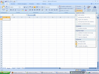
Como formatear una hoja de calculo

Para formatear una hoja de calculo es de vital importacion  tener algunos pasos claros:

1. Abrir la hoja en donde va a trabajar 
2. Dirigirse a la opcion de inicio. Esta opcion la podemos encontrar en la barra de opciones
3. En este paso buscamos la opcion formato y en ella podemos arreglar toda la hoja de calculo

Como formatear una celda

 

Con estas imagenes podremos explicar como formatear una celda en esta primera podemos observar que el primer paso para formatear la celda es hacer clik derecho y enseguida una ventanita nos aparece con muchas opciones, en esa ventanita nos dirigimos a escojer una que dice FORMATO DE CELDA, en esa opcion le damos clik  

 

En el siguiente paso instantaneamente otra ventana se nos abre con mas opciones y ya aqui podemos escojes el tipo de formato que le vamos a dar a nuestra celda